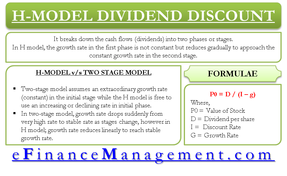
The H model is another form of the Dividend Discount Model under Discounted Cash flow (DCF) method, which breaks down the cash flows (dividends) into two phases or stages. It is similar, or one can say, a variation of a two-stage model; however, unlike the classical two-stage model, this model differs in how the growth rates are defined in the two stages.
The two-stage model assumes that the first stage goes through an extraordinary growth phase while the second stage goes through a constant growth phase. In the H model, the growth rate in the first phase is not constant but reduces gradually to approach the constant growth rate in the second stage. The key point to note here is that the growth rate is assumed to reduce linearly in the initial phase until it reaches a stable growth rate in the second stage. The model also assumes that dividend payout and cost of equity remain constant. Let us take an example illustrating firm value using the H model dividend discount model.
Example of Valuation using H Model – Dividend Discount Model
Let us take an example of a company ABC Ltd. that has paid a dividend of $ 4 this year. Assuming a growth for the next 3 years at 13%, 10%, and 7%, respectively, in the first stage and stable growth of 4% thereafter, let us calculate the firm value using the H model dividend discount model.
The dividend values will be as follows:
Current Dividend = $ 4.00
Dividend after 1st year will be = $ 4.52 ($ 4.00 x 1.13 – growing at 13 %)
2nd year will be = $ 4.972 ($ 4.52 x 1.10 – growing at 10%)
3rd year will be = $ 5.32 ($ 4.972 x 1.07 – growing at 7%)
The dividend declared after the first stage will be $ 5.32 as calculated above.
Assuming a stable growth rate of 4% in the second stage; the dividend value after 4th year will be
$ 5.32 x 1.04 = $ 5.5328.
Assuming this as the constant dividend for the rest of the life of the company, we arrive at the present values as follows.
P0 = D/ (i – g)
Where, P0 = Value of the stock/equity
D = per-share dividend paid by the company at the end of each year
i = discount rate, which is the required rate of return that an investor wants for the risk associated with the investment in equity as against investment in risk-free security.
g = growth rate
Now using the formula for calculating the value of the firm, we can arrive at the present value at the end of 3rd year for all future cash flows as follows:
Value = $ 5.5328 / (10% – 4%)
= $ 92.21
Assuming a constant discount rate of 10%, the firm’s value can now be calculated as the present value of future cash flows.
| Tenor | Cash Flow | Discount Rate | Present Value |
| 1 | 4.52 | 10% | 4.11 |
| 2 | 4.972 | 10% | 4.11 |
| 3 | 5.32 | 10% | 3.99 |
| 3 | 92.21 | 10% | 69.28 |
| Total Present Value | 81.49 |
Present value calculations arrived as follows:
$ 4.11 = $ 4.52 / (1 + 10%) ^1
$ 4.11 = $ 4.972 / (1 + 10%) ^2
$ 5.32 = $ 5.32 / (1 + 10%) ^3
$ 69.28 = $ 92.21 / (1 + 10%) ^3
The sum of all the present values will be the value of the firm, which in our example comes to $81.49.
The H model tries to do away with some of the problems/shortcomings associated with the classical two-stage model; let us have a comparative look to better understand the H Model.
H Model V/s Two-Stage Model
- The classical two-stage model assumes an extraordinary growth rate (constant) in the initial stage. In contrast, the H model is free to use an increasing or declining rate in the initial phase and then aligns itself with the constant second-stage growth rate.
- In the two-stage model, the growth rate drops suddenly from a very high rate to a stable rate as stages change. However, in the H model, the growth rate reduces linearly to reach a stable growth rate, thereby avoiding any sudden jumps or falls.
- Like the two-stage model, the H model also assumes a constant dividend payout ratio and cost of equity which may not be a real-world scenario and may lead to estimation errors.
The main limitation of the H Model is that it assumes a linear fall in growth rates from an extraordinary growth rate period in stage 1 to a stable growth rate period in stage 2.
Some of the limitations can be handled by using the 3 stage model. A 3 stage model assumes 1st stage to have an extraordinarily high rate of growth, the second stage has a reducing growth rate, and the third stage has a constant stable growth rate. One can say that it is a blend of the two-stage model and the H model.
Also Read: Cost of Equity – Dividend Discount Model
In cases where the transition happens faster from the extraordinary phase to the stable growth rate phase, a three-stage model may behave the same as in the same way as the H model, and so would the value of the firm using either model. As a result, many cases for the H model yield similar results as the three stages model.