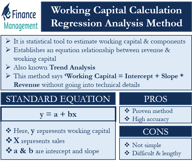
Regression analysis is a statistical tool to estimate the working capital and its components. It establishes an equation relationship between revenue and working capital. It can also be called trend analysis because the relation is carved out based on past trends. This method says ‘Working Capital = Intercept + Slope * Revenue without going into technical details.’ Let us see in detail about working capital calculation.
The standard equation is stated as below:
y = a + bx
In our case, y represents the working capital because that is to be forecasted. X represents sales as it is the base for finding out the working capital. a & b are intercept and slope. A slope is the rate of change of working capital with one unit change in revenue. Intercept is the point where the regression line and working capital axis meet. At the end of the statistical exercise with past revenue and working capital data, we will get an equation as explained above with real values of a and b. Then we will be able to find out y (working capital) for a given x (forecasted sales).

How to Calculate Working Capital using Regression Analysis with Formula and Example
Let us understand what we have to do to get our estimates rather than understanding too much technical statistics. See the following table. The first column is a year, the second is sales, and the third is working capital. As we required the past data for future forecasting, here we have our past data. The fourth column is the product of sales and working capital, and the fifth is the square of sales.
| Sr. No. | Year | Sales | Working Capital | Product of Sales & WC | Square of Sales (x) |
| (x) | (y) | x*y | x2 | ||
| 1 | 2001 | 100 | 55 | 5500 | 10000 |
| 2 | 2002 | 110 | 64 | 7040 | 12100 |
| 3 | 2003 | 121 | 80 | 9680 | 14641 |
| 4 | 2004 | 130 | 70 | 9100 | 16900 |
| 5 | 2005 | 150 | 90 | 13500 | 22500 |
| 6 | 2006 | 180 | 120 | 21600 | 32400 |
| 7 | 2007 | 181 | 100 | 18100 | 32761 |
| 8 | 2008 | 190 | 140 | 26600 | 36100 |
| 9 | 2009 | 230 | 150 | 34500 | 52900 |
| 10 | 2010 | 250 | 160 | 40000 | 62500 |
| Gross | 10 | 1642 | 1029 | 185620 | 292802 |
| Total | Years | ||||
| Denotation | n | Σx | Σy | Σxy | Σx2 |
Once this table is ready with n, Σx, Σy, Σxy, and Σx2. We will solve the following equations.
| Formula = Σy = na + bΣx | Formula = Σxy = aΣx + bΣx2 |
| Will replace the formula with values we have | Will replace the formula with values we have |
| 1029 = 10a + 1642b | 185620 = 1642a + 292802b |
| Multiply by 1642 | Multiply by 10 |
| => 1689618 = 16420a + 2696164 ———– Eq. (1) | => 1856200 = 16420a + 2928020b ———– Eq. (2) |
| Subtract Eq. (1) from (2), we get, | |
| 166582 = 0 + 231856 b | |
| => b = 166582/231856 = 0.7185 | |
| Now, replace b = 0.7185 in our old eq. 1029 = 10a + 1642b | |
| We get, a = -15. 078 |
After all this exercise, we get the following equation,
Working Capital (x) = -15.078 + 0.7185 Sales (b)
Now, if the forecasted sales for the year 2015 are 300, the working capital as per this method would be 200.472. (Working Capital = -15.078 + 0.7185 * 300 = 200.472). Similarly, all the components can be calculated.
Advantages and Disadvantages
The advantage of this method is that it is based on regression analysis, a proven method of forecasting. The bigger the amount of data we have, the better are the chances of accuracy with this method. Its drawback is that it is not simple like the percentage of sales method. The understanding and calculation both are difficult and lengthy.
Other Methods for Estimating the Working Capital Requirements:


Very use full method